What are Riemann Sums?

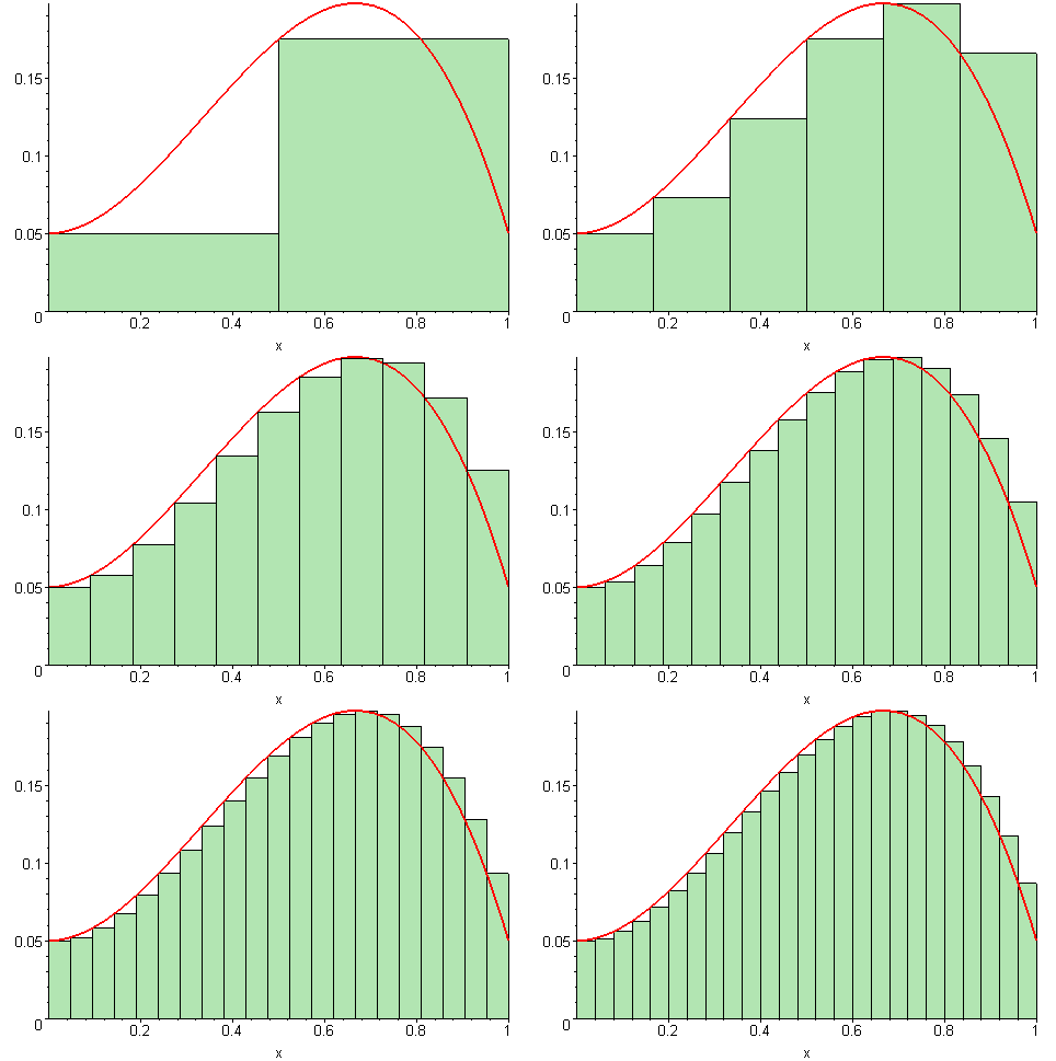
The Riemann Sum is a way of approximating the area under a curve on a certain interval [a, b] developed by Bernhard Riemann. The way a Riemann sum works is that it approximates the area by summing up the area of rectangles and then finding the area as the number of rectangles increases to infinity with an infinitely thin width. The following gif may give you a better visual example:

Riemann sums are useful because if you're dealing with a complex function, the area underneath it can be approximated with just a few rectangles. As the number of rectangles increases, you can see that the accuracy of the approximation increases. A perfect Riemann sum has infinitely many rectangles with an infinitely thin width, so of course, an infinite Riemann sum cannot be summed up by hand (unless you want to sit there for a VERY long time, and by that I mean literally forever). The formal definition of a Riemann sum is:

Woah! That looks really really scary, doesn't it? Well, it's actually quite simple, so let's break it down. The large E looking symbol, if you are unfamiliar, is the Greek letter sigma and is used for summing together a bunch of elements or numbers. This article from MathsIsFun.com can help out!

The use of sigma here makes sense since we're summing together a bunch of rectangles. Now, let's tackle the inside of the sum, the f(xk)*Δx. Remember, we're summing together the areas of rectangles, so this must be the area of some rectangle. Recall that A = bh (or alternatively A = lw) for rectangles. So one of these must be the height of our rectangles, the other must be our width.

🎥Live Stream: Reimann Sums

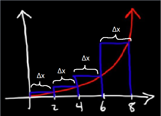
You can see in the image that Δx = (b-a)/n. What does this mean? Our area is being taken on the interval [a, b], so b-a is just the length of our interval. For example, if we were finding the area on the interval [3, 8], b - a = 5. Similarly, n is the number of rectangles we have (in a perfect Riemann sum, n approaches infinity). Therefore, (b-a)/n is the equivalent of saying we're taking our interval and chopping it up into n sized pieces on that interval. Here's a visual:

In this example, we are finding the sum from 0 to 8, so b - a = 8. We have n = 4 rectangles, so Δx = (b - a)/n = 8/4 = 2. This makes sense, we took a range of 8 and cut it into 4 equal rectangles (The rectangles in a Riemann sum will have the same width if you are just given a number of rectangles and an interval).

If Δx is the width of our rectangles, f(xk) must be the height! This makes pretty intuitive sense since, for some x value, f(x) tells you essentially the height of the graph at that x. What is k, though? k tells us essentially what rectangle we're on. So for example, at k = 1, we are looking at the first rectangle. Well, how do we find f(xk)? First, we must find xk itself. You'll see in the formula above that xk = a + kΔx. Let's think about this for a second. a is our initial value, our starting point on our interval. k is what rectangle we're on and Δx is the width of each rectangle. xk, therefore, is a way of calculating the x value of each rectangle. In this instance, we're looking at the right x value of each. If we start at k = 0, we have a left Riemann sum.

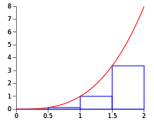
So imagine you are given this equation: f(x) = x^2. Your interval is [0,5] and n = 5. For the purposes of simplicity, I am going to demonstrate a Left Riemann Sum.

Equation: f(x) = x^2 Interval: [a,b] and in the case of this problem [1,5] - these are the parameters for the section under the curve that you are estimating N: n=4 - this number determines how many rectangles you are splitting the section under the curve into. (Note: More rectangles = more precision, but also means more work)

The top left (for a Left Riemann Sum) corner of each rectangle meets the curve (If you were to take a Right Riemann Sum you would use the top right corner of each rectangle and if you were to use a Midpoint Riemann Sum the height would be where the middle of each rectangle hit the curve)

Our heights for this specific problem would be 1, 4, 9, and 16 

(1)(1) + (1)(4) + (1)(9) + (1)(16) = 30

A = Δx( f(x1) + f(x2) + f(x3)...)

^In simplest terms, this equation will help you solve any Riemann Sum. Note that all the steps are the same for Right Riemann Sums except for #3. Just remember to use the top left corner of your rectangles for each Left Riemann Sum and the top right corner for each Right Riemann Sum.

For some quick background, when you use the areas of rectangles to estimate the area under a curve, that estimate is a Riemann Sum. When using this method you have two options: a Left Riemann Sum or a Right Riemann Sum. But what's the difference and when should you use each one?

In all honesty, there are no set restrictions that determine when to use each one. Neither method is strictly better than the other.  It is up to you to look at how the rectangles fit within the curve to determine whether a Right or Left Riemann Sum will provide you with a more accurate estimate, but for the most part, the AP exam will tell you which approximation to use.

👉
2012 AP Calculus BC Midpoint Reimann Sum FRQ 

You may have noticed earlier that we discussed whether or not a Riemann sum is an overapproximation or an underapproximation. This depends on two things: if the function is increasing or decreasing, and if we are using a righthand Riemann sum or a lefthand Riemann sum. If a function is increasing, lefthand is an underapproximation and righthand is an overapproximation and vice versa.

Riemann sums are an incredibly powerful tool when approximating areas, and they can even be used, when infinitesimal, to calculate exact areas. Approximating areas is useful, especially when you're dealing with a function where finding an anti-derivative is difficult or would take too long. Using Riemann sums in calculus opens up a whole new world of integration

With Reimann Sums, it is important to master all Applications of Integration.

Start reading Unit 8: Applications of Integration