2.9 Analyzing Departures from Linearity
3 min read•december 9, 2020
Peter Cao
AP Statistics 📊
265 resourcesSee Units
Sometimes, the least squares regression model may not be the best for representing a data set. We’re going to list some reasons why.
Influential Points
An influential point is a point that when added, significantly changes the regression model, whether by affecting the slope, y-intercept, or correlation. There are two types: outliers and high-leverage points, which are both shown in this graph.
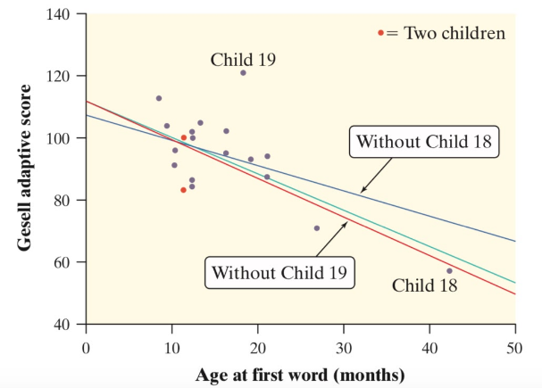
Courtesy of Starnes, Daren S. and Tabor, Josh. The Practice of Statistics—For the AP Exam, 5th Edition. Cengage Publishing.
Outliers
An outlier is a point in which the y-value is far away from the rest of the points, that is, it has a high-magnitude residual. These points heavily reduce the correlation of the scatterplot and can occasionally change the y-intercept of a regression line. Child 19 on the scatterplot above is an outlier.
High-Leverage Points
A high-leverage point is a point in which the x-value is far away from the rest of the points. These points pull the regression line towards this point, and thus can significantly change the slope of the line. It can occasionally change the y-intercept of a regression line. Child 18 on the scatterplot above is a high-leverage point.
Transforming Data and Nonlinear Regression
Sometimes, a linear model is not a good fit for a set of data, and thus it is better to use a nonlinear model. The types that we have to know for this class are exponential and power regression models. (There is also polynomial regression, but that requires knowledge of linear algebra, which is beyond the scope of this course.)
To use exponential and power regression, we will need to transform the data to linearize it (However, most calculators have options to automatically calculate this for you.).
Exponential Models
Exponential models are of the form ŷ=ab^x. We transform this by taking the natural logarithm of both sides. With logarithm properties, we get ln(ŷ)=ln(a)+ln(b)x. This means that the relationship between ln(ŷ) and x is linear, so we find the LSRL of this transformed data with the y-intercept being a* and the slope being b*. To find a and b, we use:

image courtesy of: codecogs.com

image courtesy of: codecogs.com
Power Models
Power models are of the form ŷ=ax^b. Like exponential models, we also take the natural logarithm of both sides, and with manipulation, we get ln(ŷ)=ln(a)+bln(x). This time, the relationship between ln(ŷ) and ln(x) is linear. With the LSRL of the transformer data again having y-intercept a* and slope b*, we have:

image courtesy of: codecogs.com
and b=b*.
How Can I Tell?
To evaluate which transformation to use, we check both the residual plots of the transformed data and its R^2. We pick the right model by seeing whether the residuals are randomly scattered and not curved and also whether the R^2 is close to 1. By the way, the R^2 is interpreted as the percent of variation in the response variable that can be explained by a power/exponential model relative to the explanatory variable, which is very similar to its linear counterpart. If the conditions above aren’t met, then there may be another model that may work that we haven’t learned or there are influential points skewing the data set, which is more likely.
Summary
To summarize, if our data appears to be an exponential model, we need to take the natural log (or any other base log) of our y coordinates. If our data appears to be a power model, such as a quadratic or cubic function, we need to take the log of both our x and y coordinates.
🎥Watch: AP Stats - Exploring Two-Variable Data
Browse Study Guides By Unit
👆Unit 1 – Exploring One-Variable Data
✌️Unit 2 – Exploring Two-Variable Data
🔎Unit 3 – Collecting Data
🎲Unit 4 – Probability, Random Variables, & Probability Distributions
📊Unit 5 – Sampling Distributions
⚖️Unit 6 – Proportions
😼Unit 7 – Means
✳️Unit 8 – Chi-Squares
📈Unit 9 – Slopes
✏️Frequently Asked Questions
✍️Free Response Questions (FRQs)
📆Big Reviews: Finals & Exam Prep
Fiveable
Resources
© 2023 Fiveable Inc. All rights reserved.