J
Jeanne Stansak
AP Microeconomics 🤑
95 resourcesSee Units
Introduction
I cannot stress this enough: this is quite possibly the most important unit in all of AP Micro. If there is one unit you should NOT skip, it's this one. Without further ado, let's take a look at short-run costs and cost curves!
What is the Short Run?
Before we jump in, let's discuss what we mean by "short-run."
In microeconomics we'll refer to two states of production: the short-run and the long-run. The distinction is relatively simple. In the short-run, at least one input is fixed, meaning we cannot change it. For example, a firm cannot quickly, in the short-run, build a bunch of new factories. In general, capital is considered fixed in the short-run. In the long-run, however, all bets are off and all inputs are variable. This is because given infinite time, any resource can be scaled. This guide will focus on the short run, meaning we will always have some fixed inputs, meaning some fixed costs. This will become more important later.
Fixed Costs, Variable Costs, and Total Costs
In the last guide, we quickly went over some basic terms related to costs, revenue, and profit. As a quick refresher, there are two types of costs: fixed costs and variable costs. The main difference is that fixed costs do NOT depend on output, whereas variable costs do. For example, a factory may pay for more metal for computers. This is a variable cost since the more we produce computers, the more metal we need. However, we may also pay rent on our factory. Whether we make 1, 2, 50, or 0 computers, we pay the same rent. This is a fixed cost.
We also separate costs by accounting costs and economic costs. Accounting costs are the explicit or "out of pocket" payments paid by firms to use resources during the production process. Economic costs are the sum of both the implicit costs (opportunity costs) and explicit costs of production. These costs include both the "out of pocket" payments paid by firms and the opportunity costs of using resources during the production process.
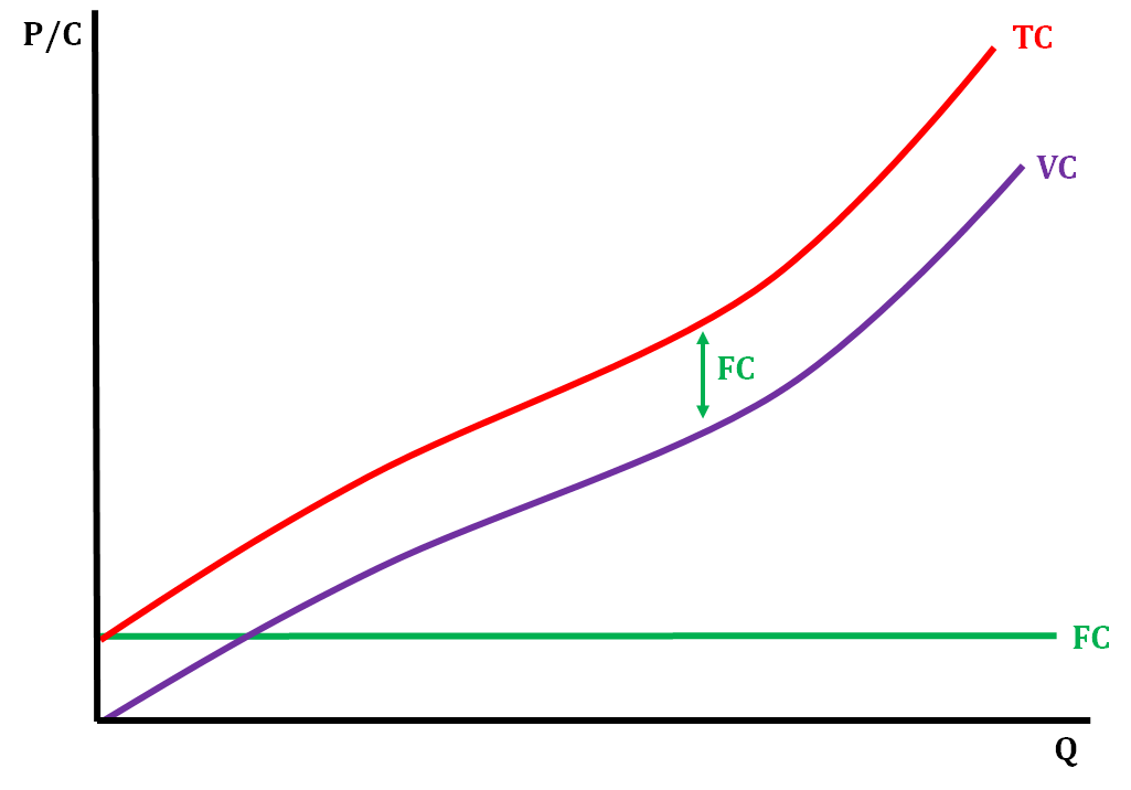
Total cost (TC) is, as the name implies, the total cost of producing some quantity of output. We can also define total cost as the sum of our variable and fixed cost. This is seen in the equation TC = FC + VC and will come in handy when we talk about average and marginal costs. When we talk about costs in economics, we are almost always talking about economic costs, but just use the word "cost". The following graph shows us what this looks like:

In this graph, we see that total cost increases as we increase quantity. This is because we spend more to produce more output. However, fixed cost stays constant, since it does not change with quantity. Also note that total cost is exactly the total variable cost shifted up by the amount of the total fixed cost.
Revenue and Profit
A firm makes revenue by selling its product. We define total revenue as price times quantity. We define profit as the difference of revenue and cost (ie. Profit = TR - TC). We have two types of profit: accounting profit and economic profit. Accounting profit only takes into account the explicit costs, whereas economic profit takes into account both explicit and implicit costs. Understanding profit as a relationship between revenue and cost will be useful as we move into perfectly competitive markets and start calculating profit.
Average and Marginal Cost Curves
Like with production, we can define the average total, fixed, and variable costs of production. This is simply done by dividing the cost by quantity to find the average cost per unit of production. They are called both average cost curves or per-unit cost curves. We have three average cost curves:
Average Total Cost (ATC) = TC / Q
Average Variable Cost (AVC) = VC / Q
Average Fixed Cost (AFC) = FC / Q
We can also quickly find one other very important identity by manipulating the first equation:
ATC = TC / Q
= (VC + FC) / Q
= (VC / Q) + (FC / Q)
= AVC + AFC
Thus, ATC = AVC + AFC. This will be clearer when we visualize these curves.
We also define marginal cost as the additional cost of producing one more unit. At first, we see diminishing marginal costs because of specialization like how we saw increasing marginal product last unit. However, because of diminishing marginal returns, we eventually see an increase in marginal cost. This leads to an upward sloping marginal cost curve.
Spoiler Alert: This upward sloping marginal cost curve has a relationship to our market supply curve. Stay tuned 😉
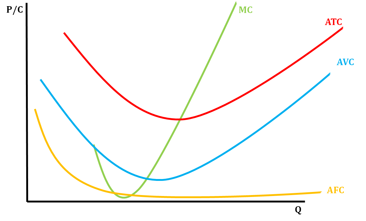
Let's take a look at what all these curves look like:

Before we explain this, let's take a breath - this is a BIG section with a lot of terms and curves, but stick with it - they're all interrelated and really intuitive!
Let's look at AFC first. Remember, AFC = FC / Q. As you may recall, fixed costs are just that - fixed! That means AFC is just some constant number divided by Q. As Q increases, FC / Q decreases until it eventually (at infinity units) reaches zero. This is why AFC is decreasing as we increase output. For those of you who are calculus people, this should feel familiar.
Next, let's break down marginal cost. Like we said before, for a short time, marginal cost is decreasing. This is because of increased specialization and increasing marginal returns. However, eventually we experience diminishing marginal returns, and as such, MC increases with quantity. The more we produce, the more the next unit costs us.
The graphs of ATC and AVC go hand and hand. They begin by decreasing, hit a minimum point when they intersect MC, and then start increasing. They begin by decreasing because marginal cost is less than ATC and AVC. When your additional cost is less than average, that drives the average down. Once marginal cost increases above ATC and AVC, the curves begin increasing.
This analogy may help: imagine you have a 4.0 GPA and you get a C in a class. This is below average, so your GPA will decrease. If you have a 2.0 GPA and get an A, your GPA will increase. If your GPA is 3.0 and you get a B (Which carries with it a GPA of 3.0), your GPA won't change. This is why ATC and AVC hit minimums when they equal MC.
For those of you who like math and are familiar with calculus, this video provides a more mathematical explanation, but this is not in the scope of AP Micro: https://www.youtube.com/watch?v=WV9vXBCHO10
Another property of these curves is that AVC approaches ATC as quantity increases. This is because as Q increases, AFC approaches zero, so the sum ATC = AVC + AFC eventually, at infinity, becomes ATC = AVC.
Example Table and Graphs

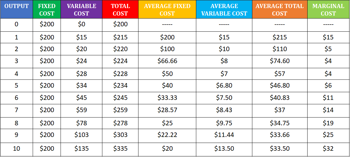
The table above shows the various cost curves of a particular firm at various levels of output. You can see at any level that Fixed Cost + Variable Cost = Total Cost. For example, at output level 6, the fixed costs are $200 and the variable costs are $45 which results in a total cost of $245. The table also shows how average fixed cost + average variable cost = average total cost. At output level 8, the AFC is $25 and the AVC is $9.75, and their sum gives you the ATC of $34.75. The final column in the table is the marginal cost (MC). Marginal cost is the change in total cost divided by the change in output, so going from an output of 2 to 3, the total cost changes from $220 to $224, and the change in output is 1 unit. This leads to a marginal cost of $4.

The diagram above shows what the FC, VC, and TC look like when graphed. The distance between the TC line and the VC line represents fixed costs. Fixed costs are constant and don't change with the production levels, but variable costs change with the level of production. Total costs change as variable costs change due to changes in output.

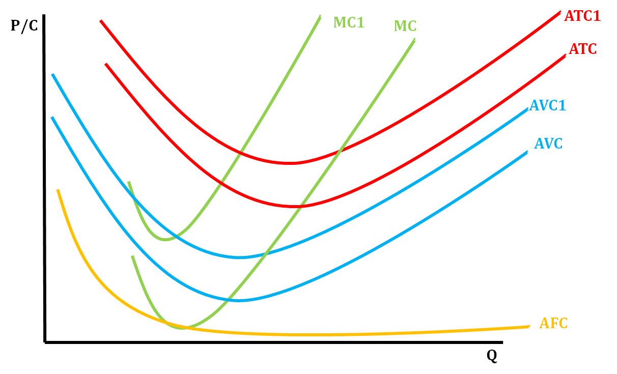
The diagram above shows how we graph marginal cost (MC), average fixed cost (AFC), average variable cost (AVC), and average total cost (ATC). MC always crosses both AVC and ATC at their lowest point. If fixed costs increase, then both the AFC and ATC would shift up and vice versa. If variable costs increase, then both AVC and ATC will shift upward and vice versa. The MC curve only shifts when variable costs change. This is because if fixed costs change, it doesn't change the additional cost of each unit. It will shift upward for an increase in variable costs and downward for a decrease in variable costs.

This graph shows what happens when all the cost curves, except for AFC, shift upward due to changes in variable costs. The opposite would happen if there was a decrease in variable costs.
Browse Study Guides By Unit
💸Unit 1 – Basic Economic Concepts
📈Unit 2 – Supply & Demand
🏋🏼♀️Unit 3 – Production, Cost, & the Perfect Competition Model
⛹🏼♀️Unit 4 – Imperfect Competition
💰Unit 5 – Factor Markets
🏛Unit 6 – Market Failure & the Role of Government
🤔Exam Skills
📚Study Tools

Fiveable
Resources
© 2025 Fiveable Inc. All rights reserved.