8.3 Carrying Out a Chi Square Goodness of Fit Test
5 min read•june 18, 2024
Jed Quiaoit
Josh Argo
AP Statistics 📊
265 resourcesSee Units
Recall from the previous section that a chi-square goodness of fit test determines if an observed frequency distribution differs significantly from a theoretical expected distribution. It is used to test whether the observed frequencies in one or more categories differ significantly from the expected frequencies in those categories. 💪
The big picture procedure for carrying out a chi-square goodness of fit test goes:
(1) Hypotheses: State the null and alternative hypotheses: The null hypothesis is that the observed frequency distribution is the same as the expected frequency distribution, while the alternative hypothesis is that the observed and expected frequency distributions are significantly different.
(2) Significance Level: Choose a significance level: This is the probability of rejecting the null hypothesis when it is true. Commonly used values are 0.1, 0.05, and 0.01.
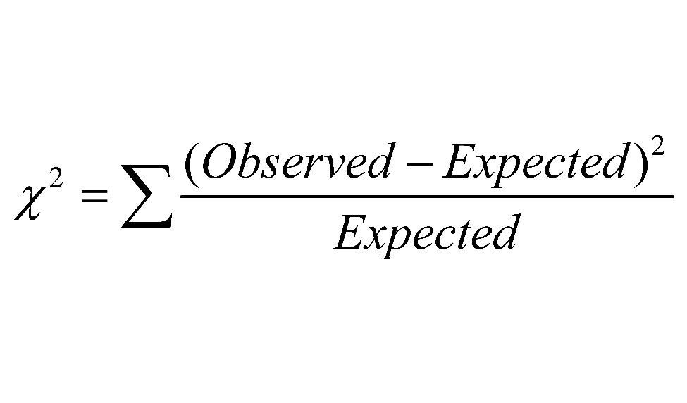
(3) Chi-Square Statistic: Calculate the chi-square statistic: The chi-square statistic is calculated using the formula:

Source: Cochrane
where "observed" is the observed frequency for each category, and "expected" is the expected frequency for each category.
(4) DF Analysis: Determine the degrees of freedom: The degrees of freedom is equal to the number of categories minus 1.
(5) Critical Value & Tables: Look up the critical value of chi-square in a chi-square table: The critical value is the value that corresponds to the chosen significance level and degrees of freedom.
(6) Comparisons! Compare the chi-square statistic to the critical value: If the chi-square statistic is greater than the critical value, then the null hypothesis is rejected and the alternative hypothesis is accepted. If the chi-square statistic is less than or equal to the critical value, then the null hypothesis cannot be rejected.
(7) Conclusion: If the null hypothesis is rejected, then the observed frequency distribution is significantly different from the expected frequency distribution. If the null hypothesis is not rejected, then the observed frequency distribution is not significantly different from the expected frequency distribution.
Doing The Test!
Now that we have checked our necessary conditions and written our hypotheses for our test, it is now time to actually carry out the test! Our test will consist of two mathematical elements: the test statistic (χ2 statistic) and our p-value. 🤖
Test Statistic
The first thing we need to calculate in order to finish our test is our χ2 value which is found using the formula found in the image above. We are going to take each of our observed counts, subtract the expected counts, square that difference and then divide by the expected count. After we have done that for all of our counts, we will sum up the total of these and get our χ2 value for that test. 📝
As with our other test statistics when we used z-scores and t-scores, a χ2 value close to 0 will support the null hypothesis, because it shows that there is not much difference between the observed and expected counts. As that difference increases more and more, we get more of an idea that our expected counts are not accurate. Therefore, leading us to reject the null hypothesis in favor of the alternate hypothesis (which states that at least one of the null proportions is incorrect).
Example
- 10% said they were unhappy (1),
- 15% said they were somewhat unhappy (2),
- 28% said they were sometimes happy and sometimes sad (3),
- 30% said they were happy (4), and
- 17% said they were always happy (5)
We take a random sample of 1000 people where 120 respond 1, 180 respond 2, 220 respond 3, 480 respond 4 and 0 respond 5.
We would:
- Take our observed counts of 120, 180, 220, 480 and 0,
- Subtract the expected counts of 100, 150, 280, 300, 170 respectively,
- Square our results;
- Divide each of the squared results by their respective expected count;
- Sum up all five of the outcomes in step 4.
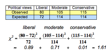
Or… use your handy, dandy, TI84 (or similar) graphing calculator to do this for you (highly recommended)! A general example of calculating chi-square values (in the context of political views in a sample of 300 people) is shown below as well.

Degrees of Freedom
As with our t-score tests and intervals, we have to find our degrees of freedom in order to complete our test. To find our degrees of freedom, we simply take the number of categories and subtract 1. So with our happiness scale example, we would have 4 degrees of freedom. ➖
P-Value
Recall that the p-value is the probability of obtaining a chi-square statistic that is at least as extreme as the one observed, given that the null hypothesis is true. 🅿️
Once you finally get your χ2 value, you calculate your p-value by finding the probability of getting that particular χ2 by random chance. As always, if our p is low, we reject the Ho.
To determine the p-value, you will need to use a chi-square table or a computer program to look up the critical value of chi-square that corresponds to the chosen significance level and degrees of freedom. The p-value is then calculated based on the observed chi-square statistic and the critical value.
Once you have calculated the chi-square statistic and p-value, you can then compare the chi-square statistic to the critical value to determine whether to reject or fail to reject the null hypothesis. If the chi-square statistic is greater than the critical value, then the null hypothesis is rejected and the alternative hypothesis is accepted. If the chi-square statistic is less than or equal to the critical value, then the null hypothesis cannot be rejected.
Example
After calculating our test for the happiness example, this was the calculator output that we got:

Conclusion
Just as we concluded hypothesis tests in previous units, we must compare our p-value to a given ɑ value. If it is less than our alpha, we conclude that we reject the H0 and have convincing evidence of the Ha. Otherwise, we fail to reject the null and do not have convincing evidence of the Ha. Remember two things:
- Never “accept” anything!
- Include context!
In the example above, we can see that our p-value is essentially 0. Therefore we would say something like this:
Since our p-value (~0) is less than 0.05, we reject the null hypothesis. We have convincing evidence that at least one of the proportions for how people rank on the happiness scale is incorrect. 😔
🎥 Watch: AP Stats Unit 8 - Chi Squared Tests
Browse Study Guides By Unit
👆Unit 1 – Exploring One-Variable Data
✌️Unit 2 – Exploring Two-Variable Data
🔎Unit 3 – Collecting Data
🎲Unit 4 – Probability, Random Variables, & Probability Distributions
📊Unit 5 – Sampling Distributions
⚖️Unit 6 – Proportions
😼Unit 7 – Means
✳️Unit 8 – Chi-Squares
📈Unit 9 – Slopes
✏️Frequently Asked Questions
📚Study Tools
🤔Exam Skills

Fiveable
Resources
© 2025 Fiveable Inc. All rights reserved.